When you have data with a header one of the most important tasks that you can do is to learn how to freeze a row in Excel. For example, if you have a header row in your data and you need to be able to scroll down but keep the header visible, so you know what you are looking at. In this tutorial I will show you how to freeze the top row and any other row that you may need to freeze.

How to Freeze the Top Row in Excel

First, we will start out with our dataset:

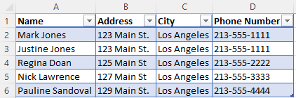
As you can see, we have a list of names, addresses, cities, and phone numbers. As this grows, we will need to keep that header information as we scroll.

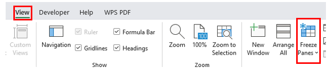
Step 1: In the ribbon click on View then click Freeze Panes:

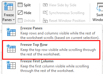
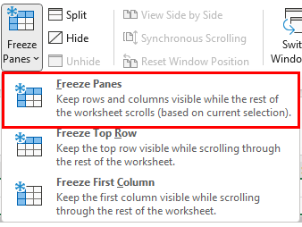
Step 2: From the drop-down menu that appears once you click on Freeze Panes click on the option to Freeze Top Row:

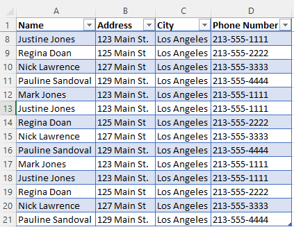
You will now be able to scroll through your spreadsheet and the top row will always be visible:

Freeze A Row Other than the Top Row

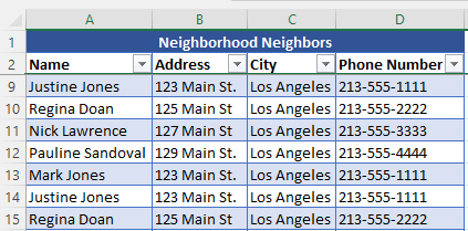
Here we will cover how to freeze a row in Excel when it is not the top row. We will use the same dataset from the previous example however this time there will be a title called Neighborhood Neighbors:

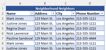
Freezing the top row in this scenario will not work since the header will scroll.

Step 1: Select the row below the line that you want to freeze. For example, in the dataset above I want to freeze under the name, address, city, and phone number header so therefore I will highlight row 3.

Step 2: In the ribbon click on View then click Freeze Panes:

Step 3: Then in the menu click on Freeze Panes:

Now the title row and header row will be displayed when you scroll as seen below:

Conclusion

Freezing rows in Excel is a common thing and therefore is beneficial to learn and to try to commit to memory. Stay tuned for tomorrow’s tutorial on how to lock cells in Excel. Until next time…