Have you ever seen a drop down list in Excel and wondered how the developer of the spreadsheet did it? Well, you’ve come to the right place. In this tutorial I will show you how to create a drop down list. We will cover the basics of how to create a drop down list in Excel such as the list itself to restricting input to only that which is on the list.

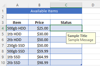
First, let’s have a look at our dataset.

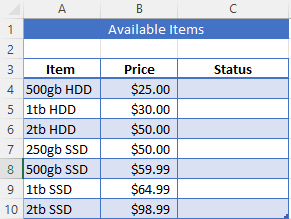
As you can see, we have some hard drives for sale and they are broken up by item, price, and status. The header a merged and centered group of three cells. If you need to know how to do that, I wrote a tutorial on how to merge cells in Excel here. What we want to do is create a drop down list in Excel under the status heading. We need to know if the item is in stock, sold, shipped, or out of stock. In order to do this we need to create a drop down list.

Step one: Click on the first cell where you will want to create a drop down list. In our case it will be cell C4.

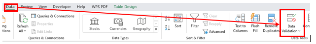
Step two: On the ribbon click on the data tab and select Data Validation under data tools.

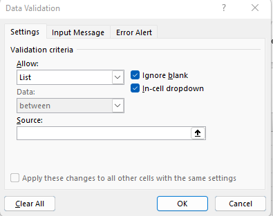
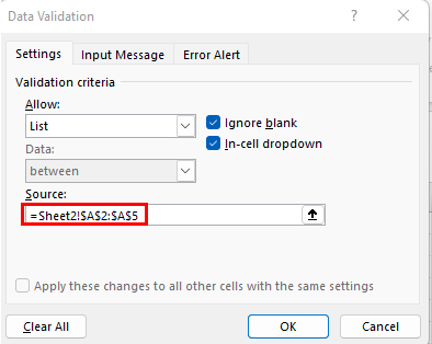
Step three: You will then see the data validation dialog box. On the settings tab it will be defaulted to Allow: Any value under Validation criteria. You will want to select List from the drop-down menu.

Once you click on list this will bring up several new options. Ignore blank will become active, In-cell dropdown is added below that and a new field called Source will display.

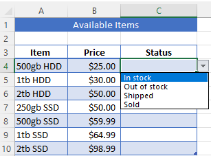
You do have a couple of different options to create your drop-down list at this point. If this is a drop-down list that you do not intend to use again, you can simply enter your choices separated by a comma as shown below:

And you can see, this will create your drop-down menu:

Should you need or want to reuse the drop down list or you are creating several drop down lists you may want to create your drop down list either in a new Excel workbook or on a separate sheet. I will walk you through creating it in the same workbook but on a different sheet

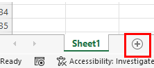
Step I: Click on the “+” sign at the bottom of the workbook.

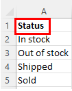
Step II: From this new sheet (default name will be Sheet2). You will then enter the selections for your drop down.

You may notice that I skipped cell A1, that was done on purpose and is a matter of personal preference. I prefer to title my drop down lists so I can simply use the name to reference them form the data validation screen.

Option 1 – Select the range of cells method: You will go back to step three above and enter the name of the new sheet that you created and the cell range of the selection for your drop down menu:

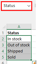
Option 2 – Name the range of cells method: You will select a name for the range of cells (I chose “Status”). Optional step: I put that name up above the range of cells so I remember the name. While this may not be necessary for one or two drop down menus, when you move to 10 or more it becomes very helpful.

Then you will select the range of cells that you are going to use for your drop down menu.

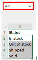
You will notice at the top to the left of the formula bar it only shows A2 as being selected. That is normal.

In that area that is showing A2 is where you will assign the range a name. I will enter in “Status” (or the name that you have selected) and press Enter. This assigns the range that name.

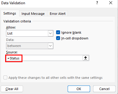
Proceed back to step 3 and in the Source enter =Status

If you want to restrict the cells to only be able to accept the in cell drop downs with the default message then at this point you will click on OK. If you want the cell(s) to accept other inputs or you want to customize the error message then continue to Step four below.

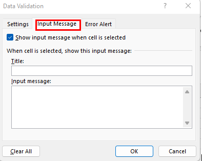
Step Four: If you would like to enter a note to show when the cell is selected, click on Input Message at the top of the Data Validation dialog box.

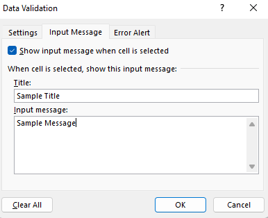
Step Five (Optional): Enter the title of the message in the Title box and the text of the message in the Input message box. Once you have entered the message and you do not want to do any more editing you can click OK:

And this is what the message will look like:

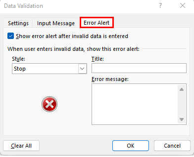
Step Six (optional): If you want to allow values other than those that are in the drop down list you have created then you will need to click on the Error Alert tab in the Data Validation dialog box.

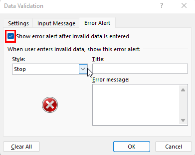
Step 7 (optional): If you want other values to be allowed in the box uncheck the box next to “Show error alert after invalid data is entered”.

Step 8 (optional): If you choose to not allow other data into the drop down list cells then you can choose a different icon under the style, either Stop, Warning, or Information.

Step Nine (Optional): You can also create a custom Title and Error message to the right.

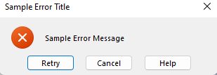
When invalid data is entered, the user will receive the error message you selected:

Conclusion

This concludes the tutorial on how to create a drop down list in Excel. Stay tuned for tomorrow’s tutorial on how to freeze a row in Excel. Until next time…