When you are working with an Excel spreadsheet there may be a time when it is necessary to learn how to merge cells in Excel. You may find yourself needing to generate a report with a title at the top that will need to be centered over several columns. Fortunately, there are several ways to merge cells together in Excel. I will be showing you two separate methods of how to merge cells in Excel below.

I must start with a word of caution; when you merge a cell it will only retain the information in the furthest, upper most cell. For example, if you wanted to merge A1-E1, only the information in A1 would be retained. Excel will however give you a warning as shown below.

Using the Ribbon

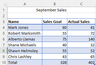
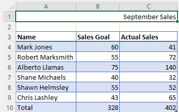
The first step that I will show you on how to merge cells in Excel is using steps that are located in the ribbon. First, we will start of with our dataset. I have used a sales team and their sales goals and actual sales for the month of September.

I want to center and merge “September Sales” across columns A1 and C1.

Step 1: Highlight cells A1- C1:

Step 2: On the Home tab in the ribbon find the Alignment section and then locate Merge & Center.

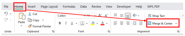
Note: You can simply click the button if you want to merge and center the item but if you want to select a different option continue to step 3.

Step 3: Click on the drop-down arrow next to Merge & Center and this will give you the following options:

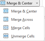
Once you select your option then your results will display. Note: I chose Merge & Center.

Using Format Cells

There is another way to merge cell in Excel that you may find beneficial. While the ribbon method does give you the ability to merge and center the format cells method allows for more control than the ribbon method allows.

Step 1: Highlight cells A1- C1:

Step 2: Right click and select Format Cells:

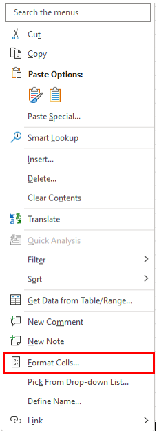
Protip: Instead of right-clicking, you can press Ctrl + 1 to bring it up as a shortcut.

Step 3: Select the Alignment tab and check Merge cells

Step 4: Under text alignment above under the Horizontal heading click on the drop-down arrow and you will have several selections:

The selections will accomplish the following actions:

General: Will merge the cells and leave the content left-aligned.

Left (Indent): Will merge the cells and leave the content left aligned.

Center: Will merge the cell and center align the content.

Right (Indent): Will merge the cells and leave the content right aligned.

Fill: Will merge the cells and repeat as long as the content can fit.

Distributed (Indent): This will push the words away from one another to fill the whole space but will be spaced evenly. For example, if there are only two words one will be right aligned and the second will be left aligned, if there are three the middle word will be centered.

Step 5: Once you have selected the alignment that you want click OK and you will see the results. I selected Right (Indent) this time.

Conclusion

While merging cells in Excel is a relatively simple task, the fact that there are so many different options does make it one of the more useful tasks to know how to complete. Stay tuned for tomorrow’s tutorial on how to create a drop-down list in Excel. Until next time…