Excel is one of the most power programs that Microsoft has created. You can track just about anything in the program and recall it at a moment’s notice. With the robust features of Excel and its tracking ability there may come times in which you will need to remove duplicate values, especially as the data that you are tracking grows in size and complexity. In this tutorial we will be covering how to remove duplicates on Excel.

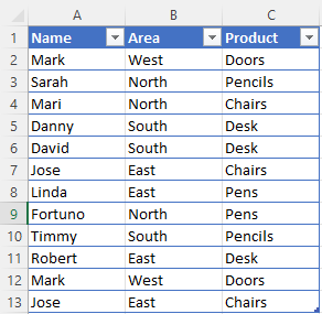
The dataset that we will be using is of a fictitious sales team. We have their name, what area that they cover, and the product that they sell.

Since the dataset is small you may notice right off that Mark/West/Doors is listed twice. At this point you could simply remove the duplicate listing but if the data that you are working with is hundreds or thousands of rows, it would be more beneficial to use Excel’s own tools to remove the duplicate(s).

Using the Remove Duplicates Tool in Excel

The first way to remove duplicates in Excel that I will cover is using the built in tools within Excel.

Step 1: Select your dataset or just one cell in your dataset.

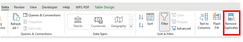
Step 2: Click on the Data tab from the header.

Step 3: Click on Remove duplicates.

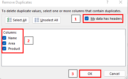
Step 4: This will bring up the Remove Duplicates menu. You will make sure that “My data has headers” is checked (it should be by default) and that what you are trying to duplicates of is checked. Once you have done this, click OK.

You will see a pop-up that indicates how many duplicate values were removed and how many remain.

Advanced Filtering

By using the advanced filtering method to remove duplicate values in Excel you will actually not be removing them from the sheet but you will be filtering them out of your results. This method is quite simple to complete.

We will once again use our original dataset

Step 1: Highlight your dataset and then click on data from the header.

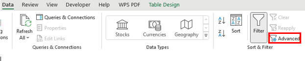
Step 2: Under the Sort & Filter options select Advanced.

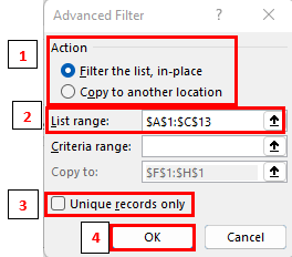
Step 3: The Advanced Filter dialog box will come up. You will select the action, Filter in place or Copy to another location. If you select Copy to another location you will be prompted to enter that location. If you did not select your dataset range you will be able to do so under List range, then you will want to select the checkbox next to Unique records only then click OK.

This will either hide the duplicate row (if you selected Filter the list, in-place) or will give you a new set of columns and rows into the area that you specified (if you selected Copy to another location).

The =COUNTIFS Formula Method

Should you want to create a formula that you can use across multiple sheets or in multiple location then maybe using a formula to remove duplicates in Excel may be the best way for you to go.

We will once again be using the original dataset from the previous method

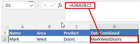
Step 1: Create a new column. Name it whatever will work for you. I called the one I created datacombined.

Step 2: You will then enter in the newly created DataCombined column the formula =A2&B2&C2

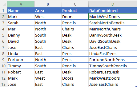
Step 3: You will then copy this down the entire column for the rows that you want to apply this to.

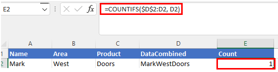
Step 4: Add another column and call it whatever you want to. It will be a count of the unique values in Column D. I called mine Count

Step 5: In that column, in cell E2, you will enter the formula =COUNTIFS ($D$2:D2,D2)

Step 6: Copy that formula down your entire dataset.

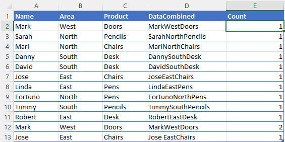
You will notice that a 2 is entered on row 12 since that is a duplicate.

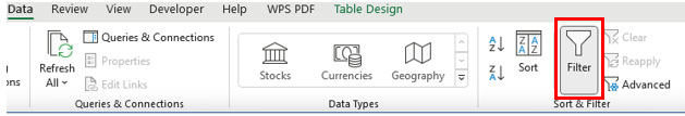
Step 7: Select your dataset and go to the data tab in the header

Step 8: Click on Filter in the Sort & Filter section of the toolbar

Step 9: In the newest column that you created (again, mine is called Count) you will click the dropdown arrow next to it and uncheck any number but the number 1

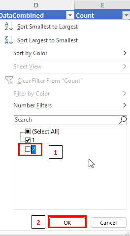
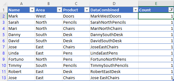
This will return only the unique values for the dataset that you are using.

BONUS: Conditional Formatting Method

While the conditional formatting method will not technically remove duplicate values in Excel, it will allow you to see which values are duplicated. This may come in handy if you wanted to see the duplicates to see if they needed to be removed or if they were ok to stay in the spreadsheet.

We will once again be using our existing dataset

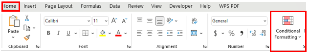
Step 1: From the home tab in the header click on Conditional Formatting in the styles section of the ribbon.

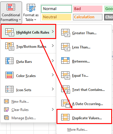
Step 2: From the Conditional Formatting menu you will select Highlight Cell Rules 🡪 Duplicate Values

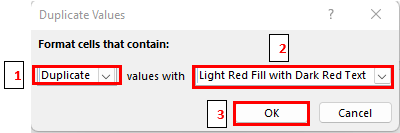
Step 3: In the Duplicate Values menu that pops up you can select duplicate or unique to be highlighted and then the value. You can also do a custom format from the menu as well. Once you have completed your selections click OK.

This will identify all of the duplicate values that appear on your dataset that you selected.

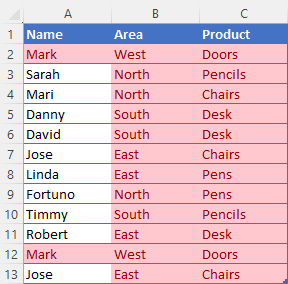
As you can see from this dataset all areas and products are duplicated but only the name Mark is duplicated.

Conclusion

While removing duplicate values in Excel can be a complicated task it is my hope that this tutorial made the task easier to accomplish and that you were able to follow along with the instructions and complete the removal of the duplicates in your dataset.

Stay tuned for tomorrow’s tutorial on how to merge cells in Excel. Until next time…