How to Lock Cells in Excel

There are times that you will need to lock a cell in Excel so that it cannot be edited, or it can only be edited by certain people. For example, you may have a calculation that you do not want someone to change the formula for or there may be data that you do not want to be changed. Regardless of the reason, I am going to show you how to lock cells in excel both with and without a password.

How to Lock A Cell in Excel

To lock a cell in Excel, you first need to unlock the entire workbook, then select the specific cell you wish to protect, and re-apply the 'Locked' protection setting to that cell. This process involves using the 'Format Cells' dialog box and then activating 'Protect Sheet' from the 'Review' tab. For enhanced security, you can also set a password to prevent unauthorized unprotection of the sheet. This tutorial will guide you through the steps to protect individual cells and optionally hide formulas, ensuring your data integrity.

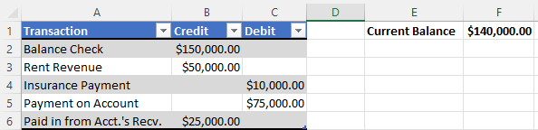
I have formatted the current balance (F1) to automatically update when an amount is entered and I do not want that formula altered.

Step 1: Select the entire workbook.

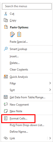
Step 2: Right click and select Format Cells.

Step 3: From the Format Cells dialog box click on the Protection tab.

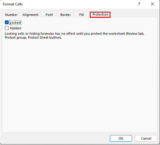
Step 4: You will notice that the Locked selection is already checked. Uncheck it and click on OK.

This will allow you to edit the rest of the spreadsheet but be able to lock a cell in Excel.

Step 5: Select the cell that you want to protect. In our dataset I have highlighted F1.

Step 6: Right click and select Format Cells.

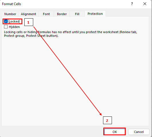
Step 7: From the Format Cells dialog box click on the Protection tab.

Step 8: You will notice that the Locked selection is not checked now since we unchecked it for the entire workbook previously. Check it and click on OK. As an option you can also check Hidden here and it will hide your formula and only show the result.

This will allow you to edit the rest of the spreadsheet but be able to lock this cell in Excel.

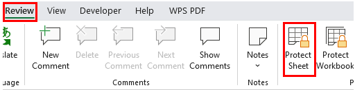
Step 9: From the ribbon select the review tab and then click on Protect Sheet.

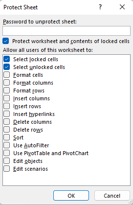
Step 10: From the Protect Sheet menu. By default, the Select locked cells and Select unlocked cells are selected. You will click OK.

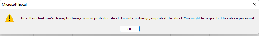
If someone should attempt to change the contents of the cell they will get an error message:

You will now notice that on the Protect Sheet area now reads Unprotect Sheet.

All a user would have to do is click on this icon and the cell(s) would be unprotected again. To avoid this we will add just one additional step.

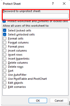
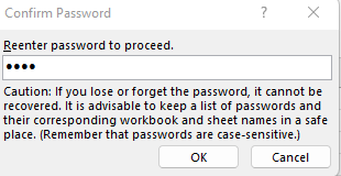
Step 11 (Optional): In step 10 there an option to enter a Password to unprotect sheet.

It will then ask you to Reenter password to proceed.

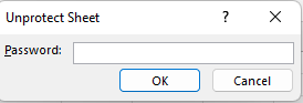
If a user were to click on Unprotect Sheet now they will be presented with a prompt to enter a password.

Conclusion

Now that I have shown you how to lock cells in Excel, how will you use it? In the meantime, stay tuned for tomorrow’s tutorial on how to remove conditional formatting in Excel. Until next time…